ReportResults
Bernard
2020-10-21
Last updated: 2020-10-21
Checks: 7 0
Knit directory: 2020_LBPcausal/
This reproducible R Markdown analysis was created with workflowr (version 1.6.2). The Checks tab describes the reproducibility checks that were applied when the results were created. The Past versions tab lists the development history.
Great! Since the R Markdown file has been committed to the Git repository, you know the exact version of the code that produced these results.
Great job! The global environment was empty. Objects defined in the global environment can affect the analysis in your R Markdown file in unknown ways. For reproduciblity it’s best to always run the code in an empty environment.
The command set.seed(20200422) was run prior to running the code in the R Markdown file. Setting a seed ensures that any results that rely on randomness, e.g. subsampling or permutations, are reproducible.
Great job! Recording the operating system, R version, and package versions is critical for reproducibility.
Nice! There were no cached chunks for this analysis, so you can be confident that you successfully produced the results during this run.
Great job! Using relative paths to the files within your workflowr project makes it easier to run your code on other machines.
Great! You are using Git for version control. Tracking code development and connecting the code version to the results is critical for reproducibility.
The results in this page were generated with repository version e8814e2. See the Past versions tab to see a history of the changes made to the R Markdown and HTML files.
Note that you need to be careful to ensure that all relevant files for the analysis have been committed to Git prior to generating the results (you can use wflow_publish or wflow_git_commit). workflowr only checks the R Markdown file, but you know if there are other scripts or data files that it depends on. Below is the status of the Git repository when the results were generated:
Ignored files:
    Ignored:    .Rhistory
    Ignored:    .Rproj.user/
    Ignored:    code/network_WIP.R
    Ignored:    code/network_WIP_mgm.R
    Ignored:    output/data_clean.xlsx
    Ignored:    output/image/
    Ignored:    output/odi_network.tiff
    Ignored:    output/odi_nw.RDS
    Ignored:    output/odi_stability.tiff
    Ignored:    output/odi_strength.tiff
    Ignored:    output/orebro_nw.RDS

Untracked files:
    Untracked:  output/temp.RData
Note that any generated files, e.g. HTML, png, CSS, etc., are not included in this status report because it is ok for generated content to have uncommitted changes.
These are the previous versions of the repository in which changes were made to the R Markdown (analysis/ReportResults.Rmd) and HTML (docs/ReportResults.html) files. If you’ve configured a remote Git repository (see ?wflow_git_remote), click on the hyperlinks in the table below to view the files as they were in that past version.
| File | Version | Author | Date | Message |
|---|---|---|---|---|
| Rmd | 71501c3 | bernard-liew | 2020-10-21 | added analysis files for publication |
Load library
# Helper packages
library (tidyverse)
library (Rgraphviz)
library (corrr)
library (corrplot)
library (DataExplorer)
library (cowplot)

# Modelling
library (bnlearn)
library (qgraph)

# Parallel
library (doParallel)

# Tables
library (flextable)
library (officer)
Import data
rm (list = ls())

load ("output/results_early2late.RData")

imp.data = impute (fit, data = df.bn, method = "bayes-lw")

var_order <- c("disability_early", "lbp_early", "lp_early", "pain_cope_early",
               "sleep_early", "work_expect_early", "pain_persist_early",
               "anx_early", "depress_early","fear_early",
               "disability_late", "lbp_late", "lp_late", "pain_cope_late",
               "sleep_late", "work_expect_late", "pain_persist_late",
               "anx_late", "depress_late","fear_late")
Descriptive plot
Mean & SD
df.plot <- df %>%
  pivot_longer(cols = -c("id", "grp", "subgrp"),
               names_to = "var",
               values_to = "val") %>%
  filter (var %in% var_order) %>%
  mutate (var = factor (var, levels = var_order),
          grp = factor (grp, labels = c("Advice", "IndvPT"))) %>%
  group_by(grp, var) %>%
  summarize (Mean = mean (val, na.rm = TRUE),
             Sd = sd (val, na.rm = TRUE))
`summarise()` regrouping output by 'grp' (override with `.groups` argument)f <- ggplot (df.plot) +
geom_point(aes (x = grp, y = Mean), colour = "black", fill = "black", stat = "identity") +
geom_errorbar(aes (x = grp, ymin = Mean - Sd, ymax = Mean + Sd), width = 0) +
facet_wrap(~ var, scales = "free") +
labs (x = "Group",
y = "Mean difference (SD)") +
theme(text = element_text(size=16)) +
theme_cowplot()
f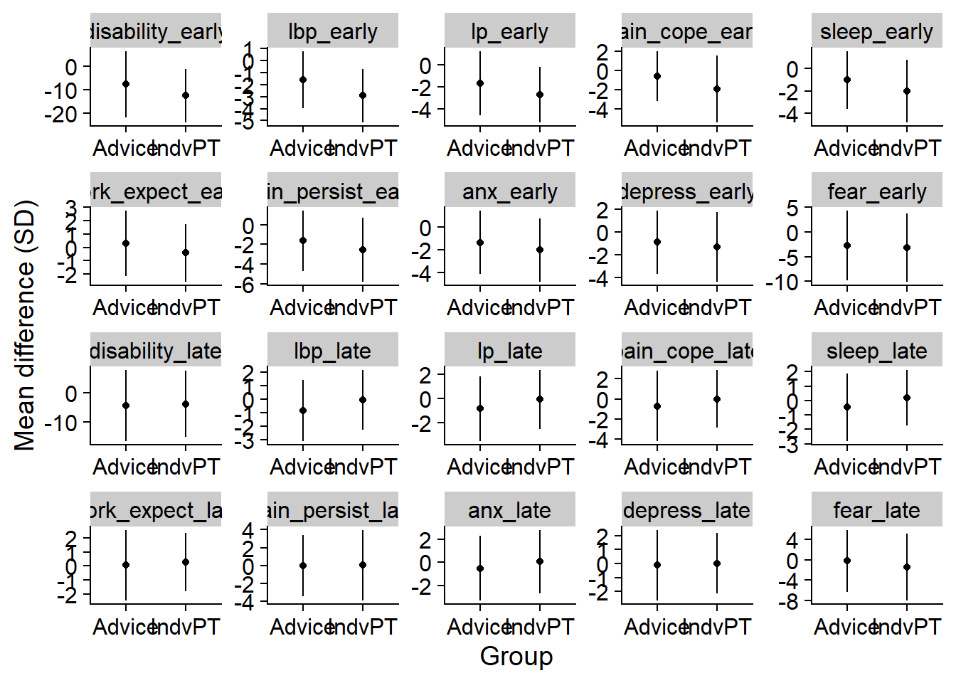
# tiff(width = 10, height = 8, units = "in", res = 100, file = "../manuscript/fig1.tiff")
# f
# dev.off()
Plot missing data of subset data
f <- plot_missing(df.bn) +
  labs (y = "Percentage missing",
        x = "Variables") +
  theme_cowplot()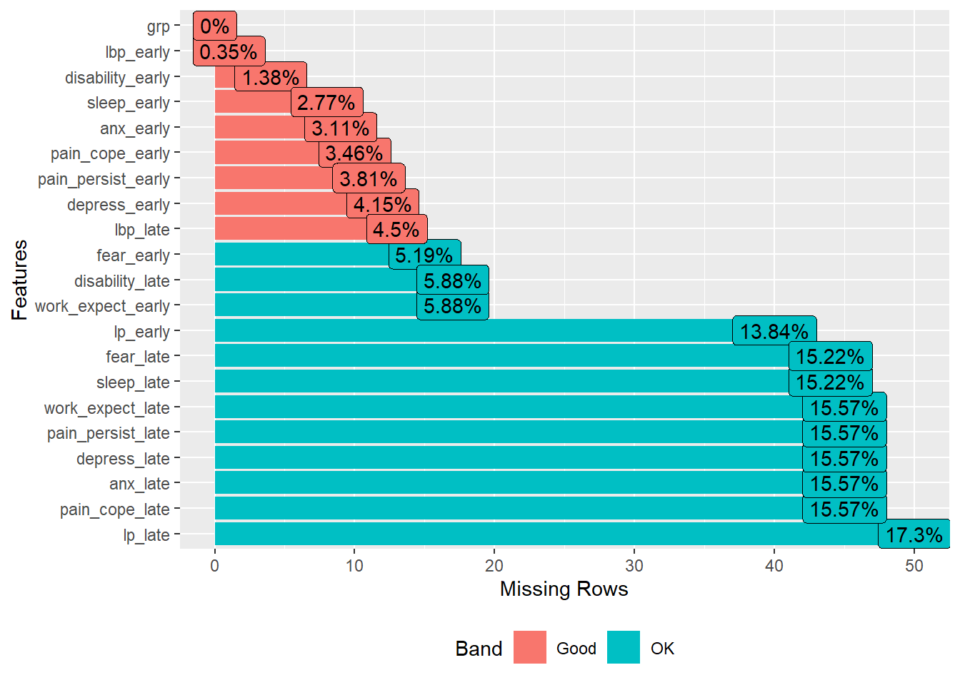
# tiff(width = 10, height = 8, units = "in", res = 300, file = "../manuscript/sm_fig1.tiff")
# f
# dev.off()
BN Results
demo.var <- c("grp")
# out.var <- grep ("outcome", names (df.bn), value = TRUE)
early.var <-  grep ("early", names (df.bn), value = TRUE)
late.var <-  grep ("late", names (df.bn), value = TRUE)

bootstr = custom.strength(boot_bl_rel, nodes = names(df.bn))
avg = averaged.network(bootstr, threshold = 0.5)
fit = bn.fit (avg, df.bn, method = "mle")

g = strength.plot(avg,
                  bootstr,
                  shape = "rectangle")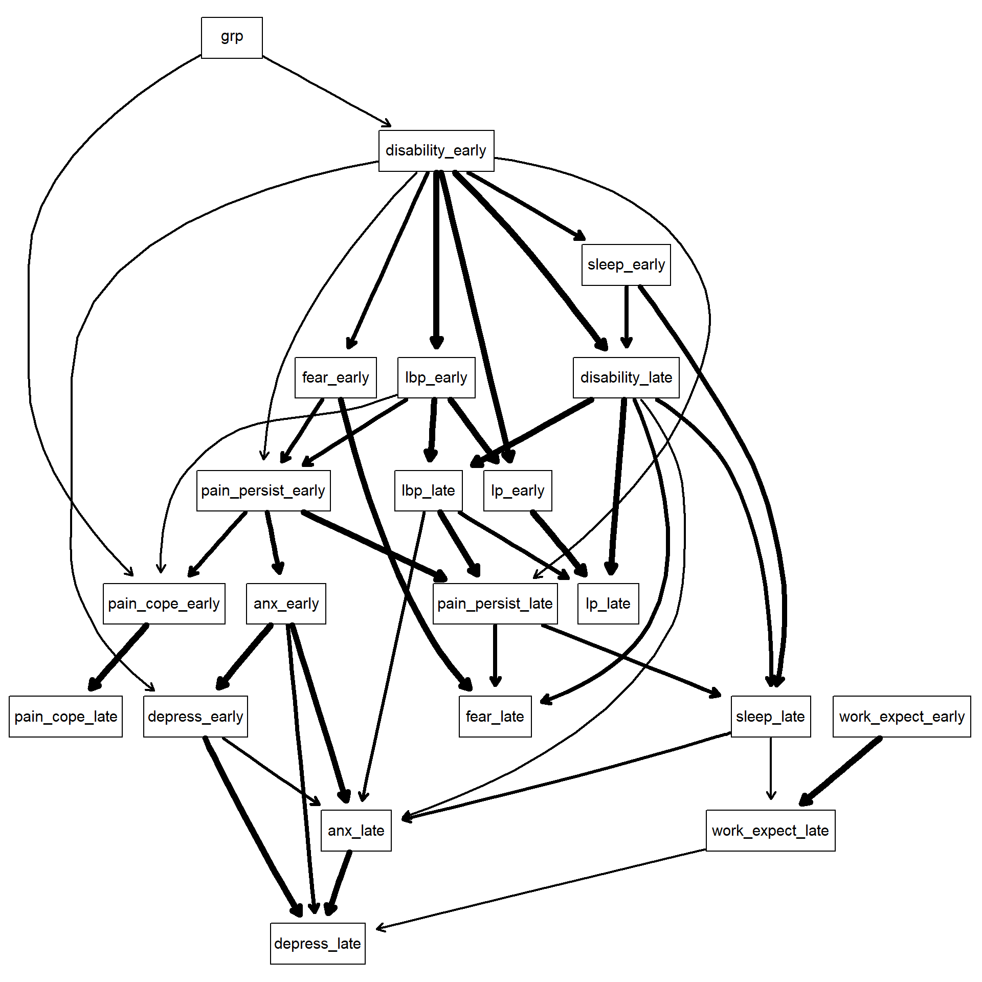
graph::nodeRenderInfo(g) = list(fontsize=18)
renderGraph(g)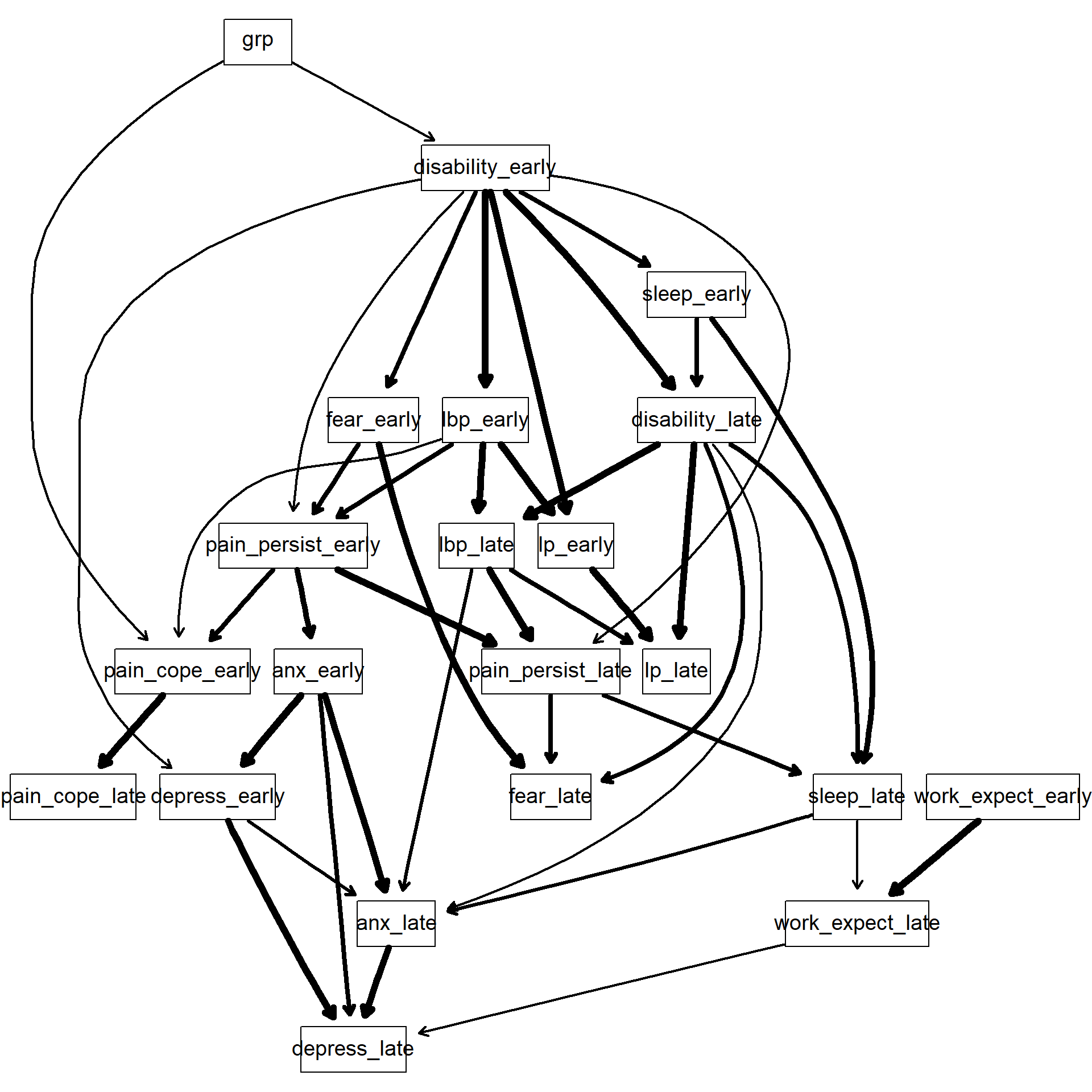
arc_col <- data.frame(arcs = names (edgeRenderInfo(g)$col)) %>%
  separate(arcs, c("parent", "child"), sep = "~")

coef_fit <- coef(fit)
coef_fit <- coef_fit[!map_lgl(coef_fit, is.matrix)]
coef_fit <- coef_fit[!map_lgl(coef_fit, is.table)]
coef_fit <-  coef_fit %>%
  unlist ()
coef_fit <- coef_fit[!grepl ("Intercept", names (coef_fit))]

coef_fit <- data.frame(arcs = names (coef_fit), coefs = coef_fit) %>%
  separate(arcs, c ("child", "parent"), sep = "[.]")

new_col <- arc_col %>%
  left_join(coef_fit, by = c("parent", "child")) %>%
  mutate (coefs = replace_na(coefs,88)) %>%
  mutate (col = ifelse (coefs < 0, "red",
                        ifelse (coefs == 88, "black", "blue"))) %>%
  mutate (col = ifelse (parent == "pain_persist_early" & child == "pain_cope_early", "blue",
                        ifelse (parent == "lbp_early" & child == "pain_cope_early", "blue", col)))

new_arc_col <- new_col$col
names (new_arc_col) <-   names (edgeRenderInfo(g)$col)

nodeRenderInfo(g)$fill[demo.var] = "cornsilk"
nodeRenderInfo(g)$fill[early.var] = "tan1"
nodeRenderInfo(g)$fill[late.var] = "gold"
#nodeRenderInfo(g)$fill[out.var] = "tomato"
edgeRenderInfo(g)$col <- new_arc_col
graph::nodeRenderInfo(g) = list(fontsize=14)


#tiff(width = 25, height = 15, units = "in", res = 300, file = "../manuscript/fig2.tiff")
renderGraph(g)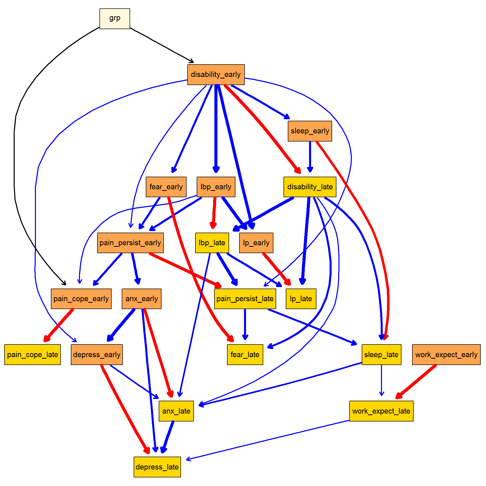
#dev.off()Correlation performance table
corr.df_ord <- corr.df[var_order]
correlation <- data.frame(Variable = names (corr.df_ord),
                          Value = corr.df_ord %>% round (2)) %>%
  mutate (Strength = ifelse (abs (Value) <= 0.3, "negligible",
                             ifelse (abs(Value) > 0.3 & abs(Value <= 0.5), "low",
                                     ifelse (abs(Value) > 0.5 & abs(Value <= 0.7), "moderate",
                                             ifelse (abs(Value) > 0.7 & abs(Value <= 0.9), "high",
                                                     "very high")))))

correlation %>%
kableExtra::kable()| Variable | Value | Strength |
|---|---|---|
| disability_early | 0.72 | high |
| lbp_early | 0.68 | moderate |
| lp_early | 0.71 | high |
| pain_cope_early | 0.52 | moderate |
| sleep_early | 0.53 | moderate |
| work_expect_early | 0.44 | low |
| pain_persist_early | 0.62 | moderate |
| anx_early | 0.76 | high |
| depress_early | 0.69 | moderate |
| fear_early | 0.55 | moderate |
| disability_late | 0.73 | high |
| lbp_late | 0.71 | high |
| lp_late | 0.70 | moderate |
| pain_cope_late | 0.46 | low |
| sleep_late | 0.59 | moderate |
| work_expect_late | 0.42 | low |
| pain_persist_late | 0.65 | moderate |
| anx_late | 0.74 | high |
| depress_late | 0.65 | moderate |
| fear_late | 0.53 | moderate |
# ft <- flextable(correlation) %>%
#       set_caption(paste0("Correlation between observed and predicted change values")) %>%
#       autofit()

# my_path <- paste0("../manuscript/table1_corr.docx")
#
# my_doc <- read_docx()  %>%
#   body_add_flextable(ft)
#
# print (my_doc, target = my_path)
Probing the expert system BN model
Evaluating the correlation between lbp_early-lbp_late relationship
See the correlation
set.seed(123)

sim <- cpdist(fit, nodes = c("lbp_early", "lbp_late"), n = 10^4,
               evidence = (TRUE))

m <- lm(lbp_late ~ lbp_early, data = sim)

coefs <- coef(m)
b0 <- round(coefs[1], 2)
b1 <- round(coefs[2],2)
r2 <- round(summary(m)$r.squared, 2)
summary (m)
Call:
lm(formula = lbp_late ~ lbp_early, data = sim)

Residuals:
    Min      1Q  Median      3Q     Max
-7.8249 -1.3806  0.0108  1.3642  7.3142

Coefficients:
             Estimate Std. Error t value Pr(>|t|)
(Intercept) -1.334012   0.027806  -47.98   <2e-16 ***
lbp_early   -0.431937   0.008416  -51.33   <2e-16 ***
---
Signif. codes:  0 '***' 0.001 '**' 0.01 '*' 0.05 '.' 0.1 ' ' 1

Residual standard error: 2.015 on 9998 degrees of freedom
Multiple R-squared:  0.2085,    Adjusted R-squared:  0.2085
F-statistic:  2634 on 1 and 9998 DF,  p-value: < 2.2e-16
eqn <- bquote(italic(lbp_late) == .(b0) + .(b1)*italic(lbp_early) * "," ~~
r^2 == .(r2))
#tiff(width = 10, height = 8, units = "in", res = 300, file = "../manuscript/fig3.tiff")
plot(sim$lbp_early, sim$lbp_late,
ylab = "Late change LBP", xlab = "Early change LBP", col = "grey", cex.axis = 1.5, cex.lab = 1.5) +
abline(coef(m), lwd = 2) +
abline(v = 0, col = 2, lty = 2, lwd = 2) +
abline(h = 0, col = 2, lty = 2, lwd = 2) +
text(x = -5, y = 5, labels = eqn, cex = 1.2)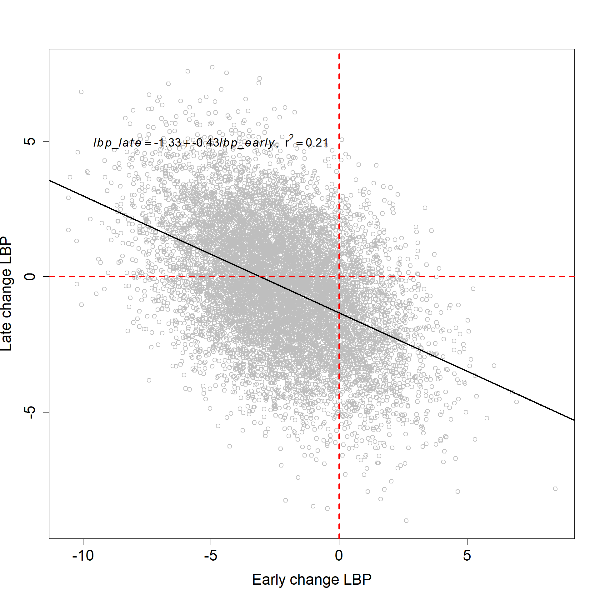
integer(0)#dev.off()Evaluating the mediating infuence of disability_early on the grp-lbp_early relationship
Influence of grp on lbp_early
set.seed(123)

sim <- cpdist(fit, nodes = c("grp", "lbp_early"), n = 10^4,
               evidence = TRUE) # individualisedphysio, advice

m <- lm(lbp_early ~ grp, data = sim)

coefs <- coef(m)
b0 <- round(coefs[1], 2)
b1 <- round(coefs[2],2)
r2 <- round(summary(m)$r.squared, 2)
summary (m)
Call:
lm(formula = lbp_early ~ grp, data = sim)

Residuals:
    Min      1Q  Median      3Q     Max
-8.6173 -1.6432 -0.0218  1.6649  9.8886

Coefficients:
                        Estimate Std. Error t value Pr(>|t|)
(Intercept)             -2.09537    0.03512 -59.657   <2e-16 ***
grpindividualisedphysio -0.41786    0.04815  -8.677   <2e-16 ***
---
Signif. codes:  0 '***' 0.001 '**' 0.01 '*' 0.05 '.' 0.1 ' ' 1

Residual standard error: 2.403 on 9998 degrees of freedom
Multiple R-squared:  0.007475,  Adjusted R-squared:  0.007376
F-statistic:  75.3 on 1 and 9998 DF,  p-value: < 2.2e-16
eqn <- bquote(italic(lp_outcome) == .(b0) + .(b1)*italic(lp_late) * "," ~~
r^2 == .(r2))
sim %>%
mutate (grp = ifelse (grp == "advice", "Advice", "IndPT")) %>%
group_by(grp) %>%
summarize (Mean = mean (lbp_early),
Sd = sd (lbp_early)) %>%
ggplot () +
geom_bar(aes (x = grp, y = Mean), color = "black", stat = "identity") +
geom_errorbar(aes (x = grp, ymin = Mean - Sd, ymax = Mean ), width = 0.2) +
labs (x = "Group",
y = "Change in early LBP") +
theme_cowplot()`summarise()` ungrouping output (override with `.groups` argument)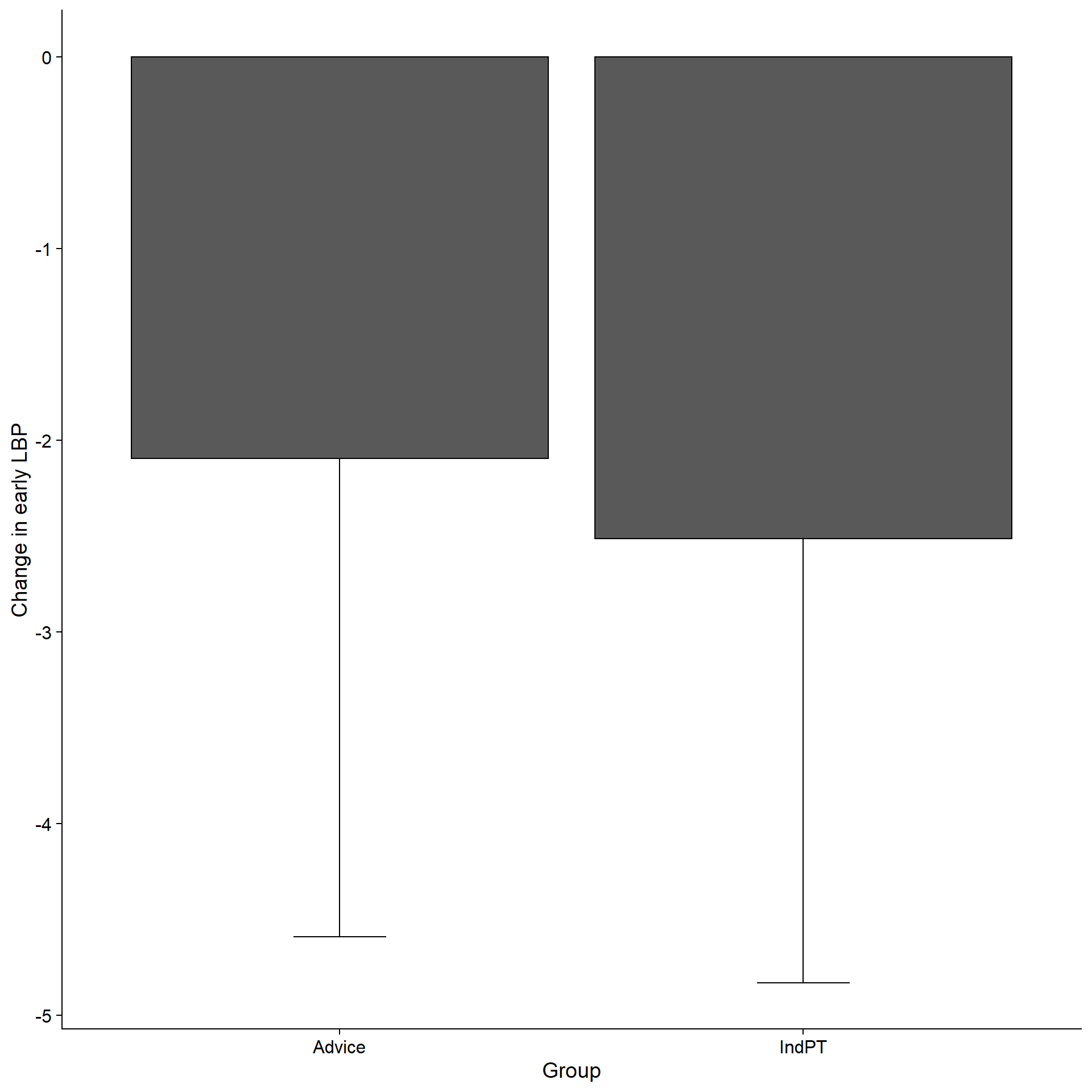
Influence of grp on lbp_early when disability_early is constant
set.seed(123)

avg.mutilated = mutilated(avg, evidence = list(disability_early = 0))

fitted.mutilated = bn.fit (avg.mutilated , df.bn, method = "mle")
fitted.mutilated$disability_early = list(coef = c("(Intercept)" = 0), sd = 0)

sim <- cpdist(fitted.mutilated, nodes = c("grp", "lbp_early"), n = 10^4,
               evidence = TRUE) # individualisedphysio, advice

m <- lm(lbp_early ~ grp, data = sim)

coefs <- coef(m)
b0 <- round(coefs[1], 2)
b1 <- round(coefs[2],2)
r2 <- round(summary(m)$r.squared, 2)
summary (m)
Call:
lm(formula = lbp_early ~ grp, data = sim)

Residuals:
   Min     1Q Median     3Q    Max
-7.073 -1.386 -0.015  1.360  8.758

Coefficients:
                        Estimate Std. Error t value Pr(>|t|)
(Intercept)             -1.31150    0.02958 -44.343   <2e-16 ***
grpindividualisedphysio  0.04672    0.04055   1.152    0.249
---
Signif. codes:  0 '***' 0.001 '**' 0.01 '*' 0.05 '.' 0.1 ' ' 1

Residual standard error: 2.023 on 9998 degrees of freedom
Multiple R-squared:  0.0001328, Adjusted R-squared:  3.277e-05
F-statistic: 1.328 on 1 and 9998 DF,  p-value: 0.2492
sim %>%
mutate (grp = ifelse (grp == "advice", "Advice", "IndPT")) %>%
group_by(grp) %>%
summarize (Mean = mean (lbp_early),
Sd = sd (lbp_early)) %>%
ggplot () +
geom_bar(aes (x = grp, y = Mean), color = "black", stat = "identity") +
geom_errorbar(aes (x = grp, ymin = Mean - Sd, ymax = Mean ), width = 0.2) +
labs (x = "Group",
y = "Change in early LBP") +
theme_cowplot()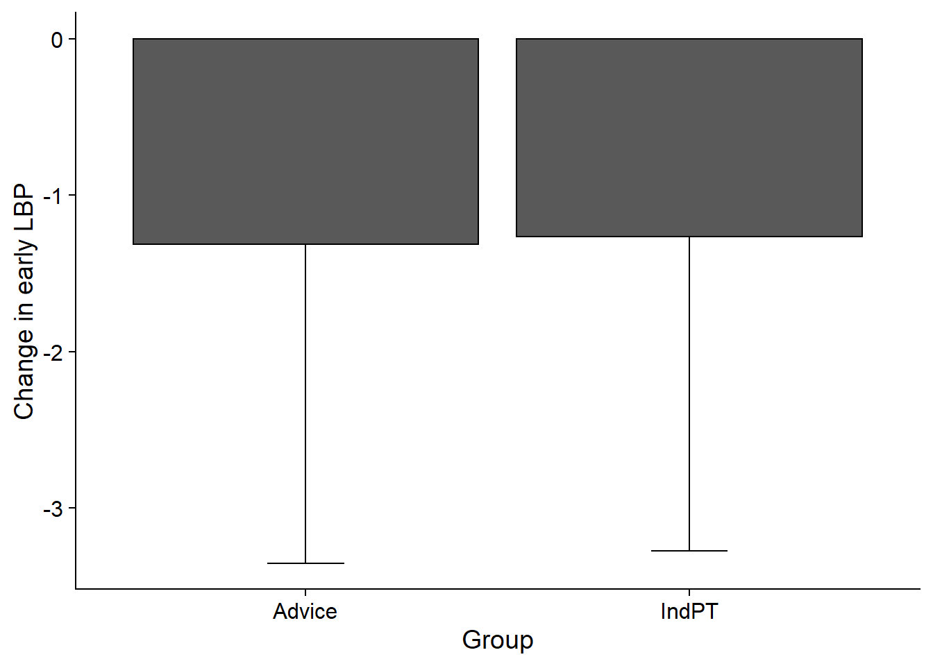
Evaluating the disability_early-depress_early relationship
See the correlation
set.seed(123)

sim <- cpdist(fit, nodes = c("disability_early", "depress_early"), n = 10^4,
               evidence = (TRUE))

m <- lm(depress_early ~ disability_early, data = sim)

coefs <- coef(m)
b0 <- round(coefs[1], 2)
b1 <- round(coefs[2],2)
r2 <- round(summary(m)$r.squared, 2)
summary (m)
Call:
lm(formula = depress_early ~ disability_early, data = sim)

Residuals:
     Min       1Q   Median       3Q      Max
-10.0691  -1.9157  -0.0429   1.9069  11.9347

Coefficients:
                  Estimate Std. Error t value Pr(>|t|)
(Intercept)      -0.632550   0.036458  -17.35   <2e-16 ***
disability_early  0.044540   0.002185   20.38   <2e-16 ***
---
Signif. codes:  0 '***' 0.001 '**' 0.01 '*' 0.05 '.' 0.1 ' ' 1

Residual standard error: 2.828 on 9998 degrees of freedom
Multiple R-squared:  0.03989,   Adjusted R-squared:  0.0398
F-statistic: 415.4 on 1 and 9998 DF,  p-value: < 2.2e-16
eqn <- bquote(italic(depress_early) == .(b0) + .(b1)*italic(disability_early) * "," ~~
r^2 == .(r2))
#tiff(width = 10, height = 8, units = "in", res = 300, file = "../manuscript/fig4.tiff")
plot(sim$disability_early, sim$depress_early, ylab = "Early change depression", xlab = "Early change disability", col = "grey", cex.axis = 1.5, cex.lab = 1.5) +
abline(coef(m), lwd = 2) +
abline(v = 0, col = 2, lty = 2, lwd = 2) +
abline(h = 0, col = 2, lty = 2, lwd = 2) +
text(x = -20, y = 6, labels = eqn, cex = 1.2)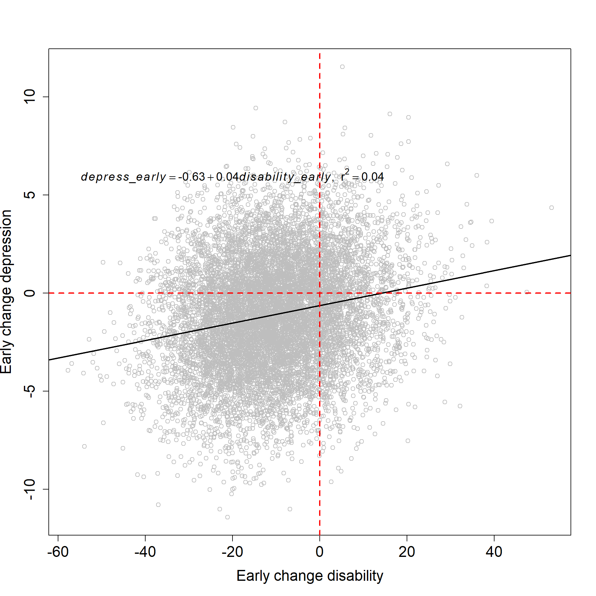
integer(0)#dev.off()Mediating influence of fear_early.
set.seed(123)

avg.mutilated = mutilated(avg, evidence = list(fear_early = 0))
fitted.mutilated = bn.fit (avg.mutilated , df.bn, method = "mle")
fitted.mutilated$fear_early= list(coef = c("(Intercept)" = 0), sd = 0)

sim <- cpdist(fitted.mutilated, nodes = c("disability_early", "depress_early"), n = 10^4,
               evidence = (TRUE))

m <- lm(depress_early ~ disability_early, data = sim)

coefs <- coef(m)
b0 <- round(coefs[1], 2)
b1 <- round(coefs[2],2)
r2 <- round(summary(m)$r.squared, 2)
summary (m)
Call:
lm(formula = depress_early ~ disability_early, data = sim)

Residuals:
     Min       1Q   Median       3Q      Max
-10.1033  -1.9252  -0.0339   1.9126  11.9575

Coefficients:
                  Estimate Std. Error t value Pr(>|t|)
(Intercept)      -0.615390   0.036416  -16.90   <2e-16 ***
disability_early  0.041966   0.002183   19.23   <2e-16 ***
---
Signif. codes:  0 '***' 0.001 '**' 0.01 '*' 0.05 '.' 0.1 ' ' 1

Residual standard error: 2.824 on 9998 degrees of freedom
Multiple R-squared:  0.03566,   Adjusted R-squared:  0.03556
F-statistic: 369.7 on 1 and 9998 DF,  p-value: < 2.2e-16
Mediating influence of lbp_early.
set.seed(123)

avg.mutilated = mutilated(avg, evidence = list(lbp_early = 0))
fitted.mutilated = bn.fit (avg.mutilated , df.bn, method = "mle")
fitted.mutilated$lbp_early = list(coef = c("(Intercept)" = 0), sd = 0)

sim <- cpdist(fitted.mutilated, nodes = c("disability_early", "depress_early"), n = 10^4,
               evidence = (TRUE))

m <- lm(depress_early ~ disability_early, data = sim)

coefs <- coef(m)
b0 <- round(coefs[1], 2)
b1 <- round(coefs[2],2)
r2 <- round(summary(m)$r.squared, 2)
summary (m)
Call:
lm(formula = depress_early ~ disability_early, data = sim)

Residuals:
     Min       1Q   Median       3Q      Max
-10.0558  -1.9166  -0.0348   1.9094  12.0480

Coefficients:
                  Estimate Std. Error t value Pr(>|t|)
(Intercept)      -0.558694   0.036407  -15.35   <2e-16 ***
disability_early  0.038628   0.002182   17.70   <2e-16 ***
---
Signif. codes:  0 '***' 0.001 '**' 0.01 '*' 0.05 '.' 0.1 ' ' 1

Residual standard error: 2.824 on 9998 degrees of freedom
Multiple R-squared:  0.03039,   Adjusted R-squared:  0.03029
F-statistic: 313.3 on 1 and 9998 DF,  p-value: < 2.2e-16
Mediating influence of pain_persist_early.
set.seed(123)

avg.mutilated = mutilated(avg, evidence = list(pain_persist_early = 0))
fitted.mutilated = bn.fit (avg.mutilated , df.bn, method = "mle")
fitted.mutilated$pain_persist_early = list(coef = c("(Intercept)" = 0), sd = 0)

sim <- cpdist(fitted.mutilated, nodes = c("disability_early", "depress_early"), n = 10^4,
               evidence = (TRUE))

m <- lm(depress_early ~ disability_early, data = sim)

coefs <- coef(m)
b0 <- round(coefs[1], 2)
b1 <- round(coefs[2],2)
r2 <- round(summary(m)$r.squared, 2)
summary (m)
Call:
lm(formula = depress_early ~ disability_early, data = sim)

Residuals:
     Min       1Q   Median       3Q      Max
-10.3899  -1.8847  -0.0044   1.8833  11.2537

Coefficients:
                  Estimate Std. Error t value Pr(>|t|)
(Intercept)      -0.439643   0.035721  -12.31   <2e-16 ***
disability_early  0.027573   0.002141   12.88   <2e-16 ***
---
Signif. codes:  0 '***' 0.001 '**' 0.01 '*' 0.05 '.' 0.1 ' ' 1

Residual standard error: 2.77 on 9998 degrees of freedom
Multiple R-squared:  0.01632,   Adjusted R-squared:  0.01622
F-statistic: 165.8 on 1 and 9998 DF,  p-value: < 2.2e-16
Mediating influence of fear_early, lbp_early, pain_persist_early
set.seed(123)

avg.mutilated = mutilated(avg, evidence = list(fear_early = 0, lbp_early = 0,  pain_persist_early = 0))
fitted.mutilated = bn.fit (avg.mutilated , df.bn, method = "mle")
fitted.mutilated$fear_early = list(coef = c("(Intercept)" = 0), sd = 0)
fitted.mutilated$lbp_early = list(coef = c("(Intercept)" = 0), sd = 0)
fitted.mutilated$pain_persist_early = list(coef = c("(Intercept)" = 0), sd = 0)


g = strength.plot(avg.mutilated,
                  bootstr,
                  shape = "rectangle")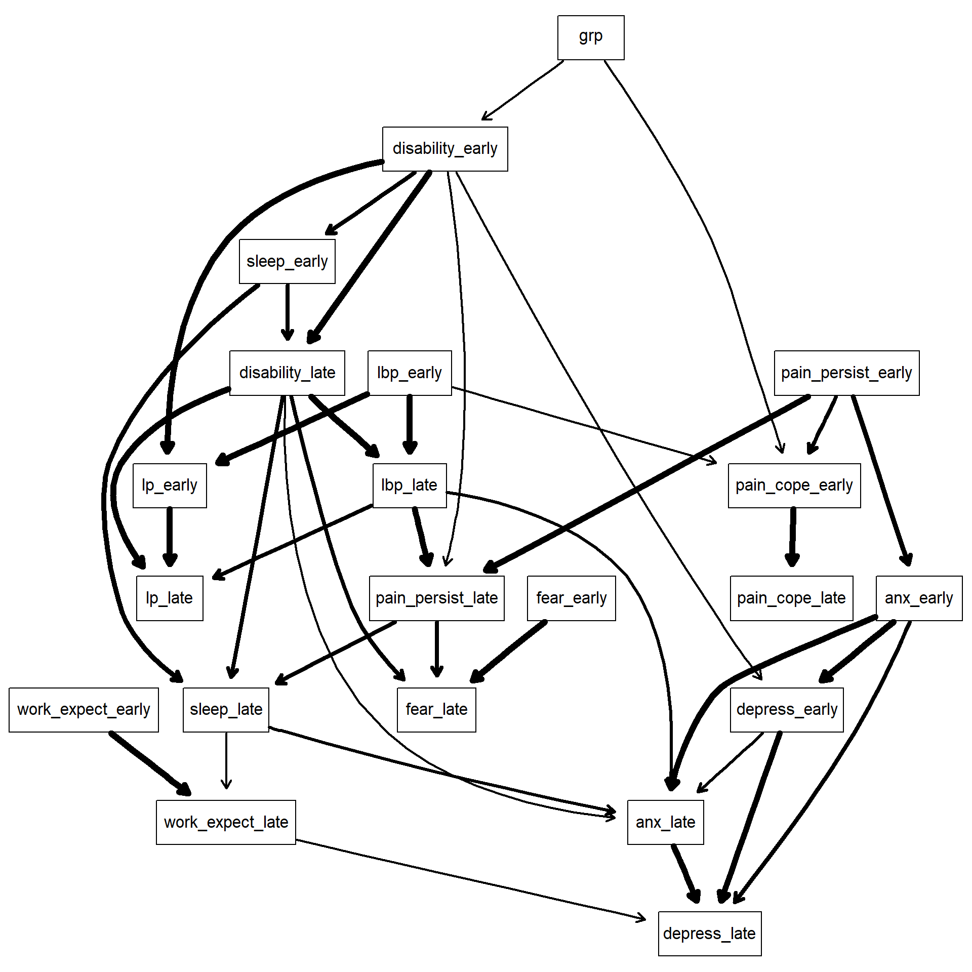
graph::nodeRenderInfo(g) = list(fontsize=18)
renderGraph(g)
sim <- cpdist(fitted.mutilated, nodes = c("disability_early", "depress_early"), n = 10^4,
               evidence = (TRUE))

m <- lm(depress_early ~ disability_early, data = sim)

coefs <- coef(m)
b0 <- round(coefs[1], 2)
b1 <- round(coefs[2],2)
r2 <- round(summary(m)$r.squared, 2)
summary (m)
Call:
lm(formula = depress_early ~ disability_early, data = sim)

Residuals:
     Min       1Q   Median       3Q      Max
-11.1248  -1.8079  -0.0121   1.7921  11.4957

Coefficients:
                  Estimate Std. Error t value Pr(>|t|)
(Intercept)      -0.437358   0.035500  -12.32   <2e-16 ***
disability_early  0.024434   0.002132   11.46   <2e-16 ***
---
Signif. codes:  0 '***' 0.001 '**' 0.01 '*' 0.05 '.' 0.1 ' ' 1

Residual standard error: 2.752 on 9998 degrees of freedom
Multiple R-squared:  0.01296,   Adjusted R-squared:  0.01286
F-statistic: 131.3 on 1 and 9998 DF,  p-value: < 2.2e-16
sessionInfo()R version 3.6.2 (2019-12-12)
Platform: x86_64-w64-mingw32/x64 (64-bit)
Running under: Windows 10 x64 (build 18363)
Matrix products: default
locale:
[1] LC_COLLATE=English_United Kingdom.1252
[2] LC_CTYPE=English_United Kingdom.1252
[3] LC_MONETARY=English_United Kingdom.1252
[4] LC_NUMERIC=C
[5] LC_TIME=English_United Kingdom.1252
attached base packages:
[1] grid parallel stats graphics grDevices utils datasets
[8] methods base
other attached packages:
[1] officer_0.3.12 flextable_0.5.10 doParallel_1.0.15
[4] iterators_1.0.12 foreach_1.5.0 qgraph_1.6.5
[7] bnlearn_4.5 cowplot_1.0.0 DataExplorer_0.8.1
[10] corrplot_0.84 corrr_0.4.2 Rgraphviz_2.30.0
[13] graph_1.64.0 BiocGenerics_0.32.0 forcats_0.5.0
[16] stringr_1.4.0 dplyr_1.0.1 purrr_0.3.4
[19] readr_1.3.1 tidyr_1.1.1 tibble_3.0.3
[22] ggplot2_3.3.2 tidyverse_1.3.0 workflowr_1.6.2
loaded via a namespace (and not attached):
[1] readxl_1.3.1 uuid_0.1-4 backports_1.1.7
[4] Hmisc_4.4-1 BDgraph_2.62 systemfonts_0.2.3
[7] plyr_1.8.6 igraph_1.2.5 splines_3.6.2
[10] digest_0.6.25 htmltools_0.5.0 fansi_0.4.1
[13] magrittr_1.5 checkmate_2.0.0 cluster_2.1.0
[16] modelr_0.1.8 jpeg_0.1-8.1 colorspace_1.4-1
[19] blob_1.2.1 rvest_0.3.6 haven_2.3.1
[22] xfun_0.16 crayon_1.3.4 jsonlite_1.7.0
[25] survival_3.2-3 glue_1.4.1 kableExtra_1.1.0
[28] gtable_0.3.0 webshot_0.5.2 abind_1.4-5
[31] scales_1.1.1 DBI_1.1.0 Rcpp_1.0.5
[34] viridisLite_0.3.0 htmlTable_2.0.1 foreign_0.8-72
[37] Formula_1.2-3 stats4_3.6.2 htmlwidgets_1.5.1
[40] httr_1.4.2 RColorBrewer_1.1-2 lavaan_0.6-7
[43] ellipsis_0.3.1 pkgconfig_2.0.3 farver_2.0.3
[46] nnet_7.3-14 dbplyr_1.4.4 tidyselect_1.1.0
[49] labeling_0.3 rlang_0.4.7 reshape2_1.4.4
[52] later_1.1.0.1 munsell_0.5.0 cellranger_1.1.0
[55] tools_3.6.2 cli_2.0.2 generics_0.0.2
[58] broom_0.7.0 fdrtool_1.2.15 evaluate_0.14
[61] yaml_2.2.1 knitr_1.29 fs_1.5.0
[64] zip_2.1.0 glasso_1.11 pbapply_1.4-3
[67] nlme_3.1-142 whisker_0.4 xml2_1.3.2
[70] compiler_3.6.2 rstudioapi_0.11 png_0.1-7
[73] reprex_0.3.0 huge_1.3.4.1 pbivnorm_0.6.0
[76] stringi_1.4.6 highr_0.8 gdtools_0.2.2
[79] lattice_0.20-41 Matrix_1.2-18 psych_2.0.7
[82] vctrs_0.3.2 pillar_1.4.6 lifecycle_0.2.0
[85] networkD3_0.4 data.table_1.13.0 corpcor_1.6.9
[88] httpuv_1.5.4 R6_2.4.1 latticeExtra_0.6-29
[91] promises_1.1.1 gridExtra_2.3 codetools_0.2-16
[94] MASS_7.3-51.6 gtools_3.8.2 assertthat_0.2.1
[97] rprojroot_1.3-2 rjson_0.2.20 withr_2.2.0
[100] mnormt_1.5-5 hms_0.5.3 rpart_4.1-15
[103] rmarkdown_2.3 git2r_0.27.1 d3Network_0.5.2.1
[106] lubridate_1.7.9 base64enc_0.1-3