3 The Basics
Download and load packages
Packages are like your iphone apps. The iphone comes with some basic functionality, e.g. weather-app. If you wanted more, you have to download. Subsequent chapters are going to start with this code chunk. This is only needed if you are running one chapter independent from others. Notice how I am using the package called pacman. This is a package manager, which loads any package you typed into it, and if it is not available, download it automatically from CRAN and load it.
if (!require("pacman")) install.packages("pacman")
pacman::p_load(tidyverse, # All purpose wrangling for dataframes
               yarrr)
In this chapter, we’ll go over the basics of the R language and the RStudio programming environment.
3.1 The command-line (Console)
Figure 3.1: Yep. R is really just a fancy calculator.
R code, on its own, is just text. You can write R code in a new script within R or RStudio, or in any text editor. However, just writing the code won’t do the whole job – in order for your code to be executed (aka, interpreted) you need to send it to the Console.
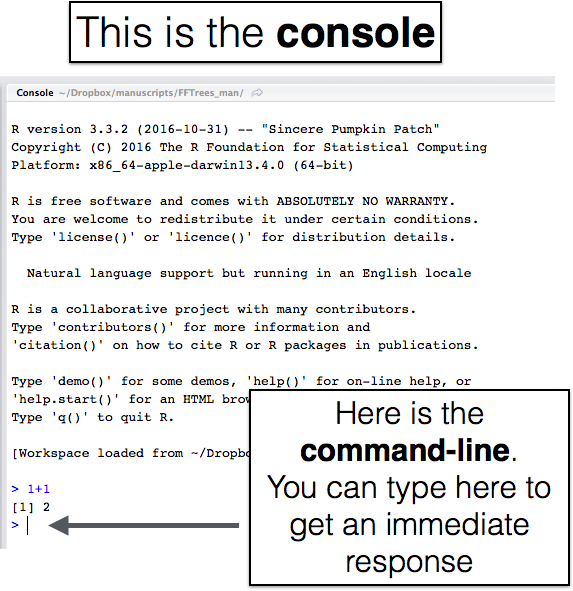
Figure 3.2: You can always type code directly into the command line to get an immediate response.
In R, the command-line interpreter starts with the > symbol. This is called the prompt. Why is it called the prompt? Well, it’s “prompting” you to feed it with some R code. The fastest way to have R evaluate code is to type your R code directly into the command-line interpreter. For example, if you type 1+1 into the interpreter and hit enter you’ll see the following
1+1## [1] 2As you can see, R returned the (thankfully correct) value of 2. You’ll notice that the console also returns the text [1]. This is just telling you you the index of the value next to it. Don’t worry about this for now, it will make more sense later. As you can see, R can, thankfully, do basic calculations. In fact, at its heart, R is technically just a fancy calculator. But that’s like saying Michael Jordan is just a fancy ball bouncer. It (and they), are much more than that.
3.2 Writing R scripts in an editor
There are certainly many cases where it makes sense to type code directly into the console. For example, to open a help menu for a new function with the ? command, to take a quick look at a dataset with the head() function, or to do simple calculations like 1+1, you should type directly into the console. However, the problem with writing all your code in the console is that nothing that you write will be saved. So if you make an error, or want to make a change to some earlier code, you have to type it all over again. Not very efficient. For this (and many more reasons), you’ll should write any important code that you want to save as an R script. An R script is just a bunch of R code in a single file. You can write an R script in any text editor, but you should save it with the .R suffix to make it clear that it contains R code.} in an editor.
In RStudio, you’ll write your R code in the Source window. To start writing a new R script in RStudio, click File – New File – R Script.
When you open a new script, you’ll see a blank page waiting for you to write as much R code as you’d like. In Figure 3.3, I have a new script called examplescript with a few random calculations.
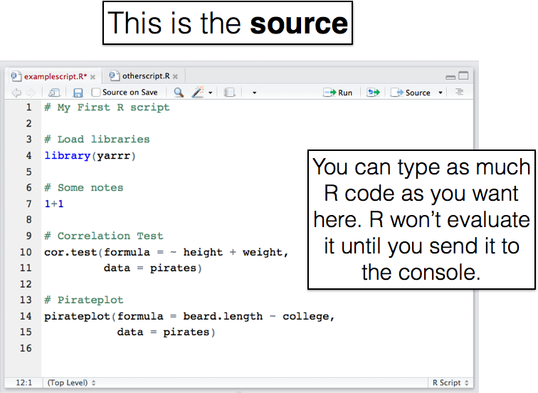
Figure 3.3: Here’s how a new script looks in the editor window on RStudio. The code you type won’t be executed until you send it to the console.
You can have several R scripts open in the source window in separate tabs (like I have above).
3.2.1 Send code from a source to the console
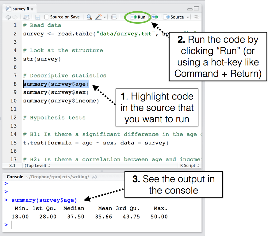
Figure 3.4: To evaluate code from the source, highlight it and run it.
When you type code into an R script, you’ll notice that, unlike typing code into the Console, nothing happens. In order for R to interpret the code, you need to send it from the Editor to the Console. There are a few ways to do this, but the most common way I use is:
- Highlight the code you want to run (with your mouse or by holding Shift), then use the Alt+Enter shortcut.
3.3 A brief style guide: Commenting and spacing
Like all programming languages, R isn’t just meant to be read by a computer, it’s also meant to be read by other humans. For this reason, it’s important that your code looks nice and is understandable to other people and your future self. To keep things brief, I won’t provide a complete style guide – instead I’ll focus on the two most critical aspects of good style: commenting and spacing.

Figure 3.5: As Stan discovered in season six of South Park, your future self is a lazy, possibly intoxicated moron. So do your future self a favor and make your code look nice. Also maybe go for a run once in a while.
3.3.1 Commenting code with the # (pound) sign
Comments are completely ignored by R and are just there for whomever is reading the code. You can use comments to explain what a certain line of code is doing, or just to visually separate meaningful chunks of code from each other. Comments in R are designated by a # (pound) sign. Whenever R encounters a # sign, it will ignore all the code after the # sign on that line. Additionally, in most coding editors (like RStudio) the editor will display comments in a separate color than standard R code to remind you that it’s a comment:
Here is an example of a short script that is nicely commented. Try to make your scripts look like this!
# Author: Pirate Jack
# Title: My nicely commented R Script
# Date: None today :(

# Step 1: Load the yarrr package
library(yarrr)

# Step 2: See the column names in the movies dataset
names(movies)

# Step 3: Calculations

# What percent of movies are sequels?
mean(movies$sequel, na.rm = T)

# How much did Pirate's of the Caribbean: On Stranger Tides make?
movies$revenue.all[movies$name == 'Pirates of the Caribbean: On Stranger Tides']
I cannot stress enough how important it is to comment your code! Trust me, even if you don’t plan on sharing your code with anyone else, keep in mind that your future self will be reading it in the future.
3.3.2 Spacing
Howwouldyouliketoreadabookiftherewerenospacesbetweenwords? I’mguessingyouwouldn’t. Soeverytimeyouwritecodewithoutproperspacing,rememberthissentence.
Commenting isn’t the only way to make your code legible. It’s important to make appropriate use of spaces and line breaks. For example, I include spaces between arithmetic operators (like =, + and -) and after commas (which we’ll get to later). For example, look at the following code:
Figure 3.6: Don’t make your code look like what a sick Triceratops with diarrhea left behind for Jeff Goldblum.
# Shitty looking code
a<-(100+3)-2
mean(c(a/100,642564624.34))
t.test(formula=revenue.all~sequel,data=movies)
plot(x=movies$budget,y=movies$dvd.usa,main="myplot")
That code looks like shit. Don’t write code like above. It wiil make your eyes hurt. Now, let’s use some liberal amounts of commenting and spacing to make it look less shitty.
# Some meaningless calculations. Not important

a <- (100 + 3) - 2
mean(c(a / 100, 642564624.34))

# t.test comparing revenue of sequels v non-sequels

t.test(formula = revenue.all ~ sequel,
       data = movies)

# A scatterplot of budget and dvd revenue.
#  Hard to see a relationship

plot(x = movies$budget,
     y = movies$dvd.usa,
     main = "myplot")
See how much better that second chunk of code looks? Not only do the comments tell us the purpose behind the code, but there are spaces and line-breaks separating distinct elements.
3.4 Objects and functions
To understand how R works, you need to know that R revolves around two things: objects and functions. Almost everything in R is either an object or a function. In the following code chunk, I’ll define a simple object called tattoos using a function c():
# 1: Create a vector object called tattoos
tattoos <- c(4, 67, 23, 4, 10, 35)

# 2: Apply the mean() function to the tattoos object
mean(tattoos)
## [1] 23.83333What is an object? An object is a thing – like a number, a dataset, a summary statistic like a mean or standard deviation, or a statistical test. Objects come in many different shapes and sizes in R. There are simple objects like the single digit 25 which represent single numbers, vectors (like our tattoos object above) which represent several numbers, more complex objects like dataframes which represent tables of data, and even more complex objects like hypothesis tests or regression which contain all sorts of statistical information.
What is a function? A function is a procedure that typically takes one or more objects as arguments (aka, inputs), does something with those objects, then returns a new object. For example, the mean() function we used above takes a vector object, like tattoos, of numeric data as an argument, calculates the arithmetic mean of those data, then returns a single number (a scalar) as a result.A great thing about R is that you can easily create your own functions that do whatever you want – but we will not get to that in the book. Thankfully, R has hundreds (thousands?) of built-in functions that perform most of the basic analysis tasks you can think of.
99% of the time you are using R, you will do the following: 1) Define objects. 2) Apply functions to those objects. 3) Repeat!. Seriously, that’s about it. However, as you’ll soon learn, the hard part is knowing how to define objects they way you want them, and knowing which function(s) will accomplish the task you want for your objects.
3.4.1 Numbers versus characters
For the most part, objects in R come in one of two flavors: numeric and character. It is very important to keep these two separate as certain functions, like mean(), and max() will only work for numeric objects, while functions like grep() and strtrim() only work for character objects.
A numeric object is just a number like 1, 10 or 3.14. You don’t have to do anything special to create a numeric object, just type it like you were using a calculator.
# These are all numeric objects
1
10
3.14
A character object is a name like "Madisen", "Brian", or "University of Konstanz". To specify a character object, you need to include quotation marks "" around the text.
# These are all character objects
"Madisen"
"Brian"
"10"
If you try to perform a function or operation meant for a numeric object on a character object (and vice-versa), R will yell at you. For example, here’s what happens when I try to take the mean of the two character objects "1" and "10":
If I make sure that the arguments are numeric (by not including the quotation marks), I won’t receive the error:
## [1] 5.53.4.2 Creating new objects with <-
By now you know that you can use R to do simple calculations. But to really take advantage of R, you need to know how to create and manipulate objects. All of the data, analyses, and even plots, you use and create are, or can be, saved as objects in R.
To create new objects in R, you need to do object assignment. Object assignment is our way of storing information, such as a number or a statistical test, into something we can easily refer to later. This is a pretty big deal. Object assignment allows us to store data objects under relevant names which we can then use to slice and dice specific data objects anytime we’d like to.
To do an assignment, we use the almighty <- operator called assign To assign something to a new object (or to change an existing object), use the notation object <- ..., where object is the new (or updated) object, and ... is whatever you want to store in object. Let’s start by creating a very simple object called a and assigning the value of 100 to it:
Good object names strike a balance between being easy to type (i.e.; short names) and interpret. If you have several datasets, it’s probably not a good idea to name them a, b, c because you’ll forget which is which. However, using long names like March2015Group1OnlyFemales will give you carpal tunnel syndrome.
# Create a new object called a with a value of 100
a <- 100
Once you run this code, you’ll notice that R doesn’t tell you anything. However, as long as you didn’t type something wrong, R should now have a new object called a which contains the number 100. If you want to see the value, you need to call the object by just executing its name. This will print the value of the object to the console:
# Print the object a
a
## [1] 100Now, R will print the value of a (in this case 100) to the console. If you try to evaluate an object that is not yet defined, R will return an error. For example, let’s try to print the object b which we haven’t yet defined:
bAs you can see, R yelled at us because the object b hasn’t been defined yet.
Once you’ve defined an object, you can combine it with other objects using basic arithmetic. Let’s create objects a and b and play around with them.
a <- 1
b <- 100

# What is a + b?
a + b
## [1] 101
# Assign a + b to a new object (c)
c <- a + b

# What is c?
c
## [1] 1013.4.2.1 To change an object, you must assign it again!
Normally I try to avoid excessive emphasis, but because this next sentence is so important, I have to just go for it. Here it goes…
To change an object, you assign it again!
No matter what you do with an object, if you don’t assign it again, it won’t change. For example, let’s say you have an object z with a value of 0. You’d like to add 1 to z in order to make it 1. To do this, you might want to just enter z + 1 – but that won’t do the job. Here’s what happens if you don’t assign it again:
z <- 0
z + 1
## [1] 1Ok! Now let’s see the value of z
z## [1] 0Damn! As you can see, the value of z is still 0! What went wrong? Oh yeah…
To change an object, you must assign it again!
The problem is that when we wrote z + 1 on the second line, R thought we just wanted it to calculate and print the value of z + 1, without storing the result as a new z object. If we want to actually update the value of z, we need to reassign the result back to z as follows:
z <- 0
z <- z + 1  # Now I'm REALLY changing z
z
## [1] 1Phew, z is now 1. Because we used assignment, z has been updated. About freaking time.
3.4.3 How to name objects
You can create object names using any combination of letters and a few special characters (like . and _). Here are some valid object names
# Valid object names
group.mean <- 10.21
my.age <- 32
FavoritePirate <- "Jack Sparrow"
sum.1.to.5 <- 1 + 2 + 3 + 4 + 5
All the object names above are perfectly valid. Now, let’s look at some examples of invalid object names. These object names are all invalid because they either contain spaces, start with numbers, or have invalid characters:
# Invalid object names!
famale ages <- 50 # spaces
5experiment <- 50 # starts with a number
a! <- 50 # has an invalid character. Anytime you see this warning in R, it almost always means that you have a naming error of some kind.
3.4.3.1 R is case-sensitive!
Figure 3.7: Like a text message, you should probably watch your use of capitalization in R.
Like English, R is case-sensitive – it R treats capital letters differently from lower-case letters. For example, the four following objects Plunder, plunder and PLUNDER are totally different objects in R:
# These are all different objects
Plunder <- 1
plunder <- 100
PLUNDER <- 5
I try to avoid using too many capital letters in object names because they require me to hold the shift key. This may sound silly, but you’d be surprised how much easier it is to type mydata than MyData 100 times.